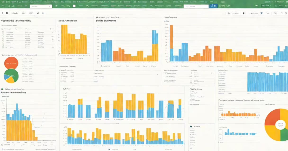
Creating a chart in Google Sheets turns raw data into visual insights using a few clicks. Select your data range, click Insert > Chart, then choose a chart type that matches your goal-like bar, line, or pie. The tool auto-generates the visual based on your selected columns and rows.
Google Sheets uses your highlighted data to determine axes, labels, and series. It supports live updates: change the underlying numbers, and the chart redraws instantly. This feature makes it ideal for tracking progress, comparing values, or presenting trends in reports.
Charts in Google Sheets are not static images-they're linked to the spreadsheet. Any edit to the source data refreshes the chart automatically. This changing behavior separates them from standalone visuals created in PowerPoint or Photoshop.
When you select a range of cells and insert a chart, Google Sheets analyzes the structure. The first row is treated as column headers unless you specify otherwise. The leftmost column becomes the horizontal axis (category axis), and each subsequent column becomes a data series.
For example, if you have monthly sales figures across three regions in columns A through D, with "Month" in A1 and region names in B1, C1, D1, Sheets recognizes this as a time-series comparison. It assigns months to the x-axis and each region's sales to a separate line or bar.
After insertion, the chart appears on the same sheet. You can move it by dragging, resize it by corner handles, or adjust its position using the Format panel on the right.
Google Sheets offers eight primary chart types. Choosing the right one depends on what you want to show:
| Chart Type | Best For | Example Use Case |
|---|---|---|
| Column | Comparing values across categories | Monthly revenue by product line |
| Bar | Showing comparisons with long category names | Team performance rankings |
| Line | Tracking changes over time | Daily website visits over 30 days |
| Pie | Displaying parts of a whole | Market share by vendor |
| Scatter | Showing relationships between two variables | Correlation between ad spend and conversion rate |
| Area | Highlighting volume over time with overlapping series | Website traffic trends across multiple channels |
| Donut | Similar to pie, but with a hole to improve readability | Expense breakdown with budget categories |
| Funnel | Visualizing stages in a process | Sales pipeline from lead to close |
Each type adapts to your data layout. A column chart works best when you have fewer than 10 categories. Too many bars clutter the view. Use a bar chart instead if labels are long.
For time-based data, line charts outperform columns. They better illustrate trends and momentum. A line chart with markers shows both direction and specific values.
One frequent error is including blank rows or merged cells in the data range. Sheets treats empty cells as zeros, which distorts the scale. Always clean your dataset before chart creation.
Another issue: misaligned headers. If your first row contains mixed data types-like dates in one cell and text in the next-Sheets may assign incorrect axes. Ensure consistent formatting. Use dates in a single column, not scattered across rows.
A lesser-known fix: disable "Show legend" if you have only one data series. The legend adds visual noise. Right-click the chart, go to Customize > Series, and uncheck "Show legend."
Suppose you track monthly sales for Q1 2024 in a sheet. Column A holds month names (January, February, March). Columns B, C, D list sales for three products: Widgets, Gears, and Tools.
Select the range A1:D4. Click Insert > Chart. Sheets defaults to a column chart. You see three bars per month, one for each product.
To improve clarity, switch to a line chart. Click the chart, then in the Chart editor, under Setup, change "Chart type" to "Line." Now you can see how each product trended over time.
Add a title: "Q1 2024 Product Sales." In Customize > Chart title, enter the text. Set font size to 16 and color to dark gray. Move the title above the chart.
Finally, adjust the y-axis scale. Right-click the vertical axis, choose "Format axis," set minimum to 0 and maximum to 1500. This prevents distortion from small differences.
The result is a clean, readable report. Anyone reviewing it can spot which product gained traction in February and which declined in March.
Google Sheets charts are not the same as pivot tables. Pivot tables summarize large datasets by grouping and aggregating. Charts visualize the results. You can't create a chart directly from a pivot table unless you copy the summarized data to a new range.
Also, don't confuse Sheets charts with embedded visuals from external tools. Google Sheets generates charts natively. They update when data changes. External images pasted into cells do not.
Another misconception: charts require complex setup. In reality, most charts take under 30 seconds to create. The default settings work for basic reporting. Fine-tuning comes later.
I once built a quarterly dashboard with 12 charts. Instead of repeatedly selecting A1:D12, I assigned the range a name-"SalesData"-via Data > Named ranges. Then, whenever I inserted a chart, I selected "SalesData" from the dropdown. This saved time and reduced errors.
Named ranges also help when sharing files. Team members see "SalesData" instead of "Sheet1!A1:D12," making the logic clearer.
Always verify the chart's source data. A mismatched range leads to misleading visuals. Check the "Data range" field in the Chart editor before finalizing.
Understanding how to make a chart in Google Sheets unlocks faster decision-making. With practice, you'll recognize the right chart type in seconds and build visuals that communicate -without needing design software.